VLOOKUP Complete Guide

What Is VLOOKUP and Why It Matters

In this VLOOKUP complete guide, you'll learn everything from basic lookups to advanced techniques. VLOOKUP (Vertical Lookup) searches for a value in the first column of a table and returns a corresponding value from another column. Think of it as Excel's built-in search engine — give it a product ID, get back the price, category, or stock level instantly. If you do reporting, reconciliation, or data merging, VLOOKUP will save you hours every week.

The syntax: =VLOOKUP(lookup_value, table_array, col_index_num, [range_lookup])

lookup_value — the cell containing what you're searching for (e.g. product ID in A2)
table_array — the full data range including both the search column and the answer column
col_index_num — which column number (counting from left of table_array) holds the answer
range_lookup — FALSE for exact match (use this 95% of the time), TRUE for approximate

VLOOKUP syntax diagram showing each argument mapped to a sample spreadsheet: lookup_value pointing to cell A2 containing 'SKU-301', table_array highlighting range B2:D100, col_index_num circled as 3 pointing to the Price column, and range_lookup showing FALSE for exact match — Fig 1. — The four VLOOKUP arguments explained visually. Notice how col_index_num counts from the left edge of your selected range, not from column A of the worksheet.

Step-by-Step: Your First VLOOKUP

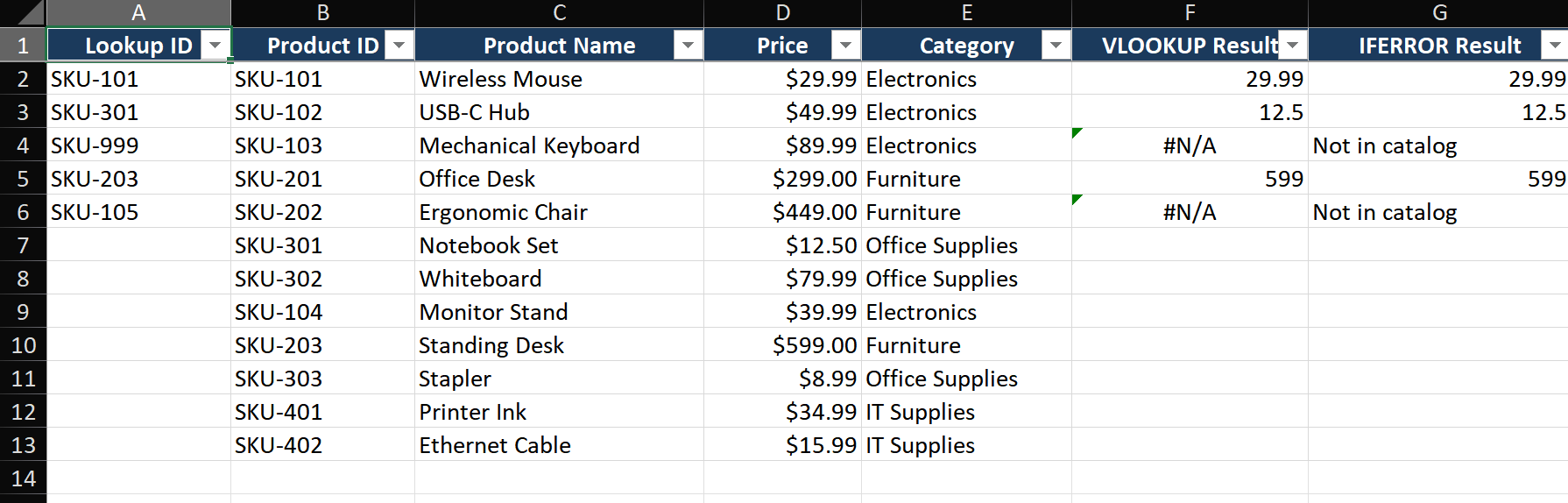
We'll walk through a real scenario. You have a product catalog in columns B through E, and in column A you have a list of product IDs to look up. You want to pull the prices from the catalog into column F.

Step 1 — Set up your data

Open your workbook and verify the data layout:

Go to your product catalog sheet. Confirm column B holds Product IDs, column D holds Prices.
Make sure there are no completely empty rows inside the catalog range. Excel treats a blank row as the end of data, which can cause VLOOKUP to miss rows below it.
Select the catalog range (B2:E500), press Ctrl+T to convert it to an Excel Table. Name it Catalog via the Table Design tab. Tables auto-expand and give you structured references.

Excel spreadsheet showing a product catalog in columns B-E: Column B 'Product ID' (B2:B12), Column C 'Product Name', Column D 'Price', Column E 'Category'. Column A shows a smaller lookup list of 5 product IDs (A2:A6). Column F is empty with header 'Lookup Result'. The catalog range B2:E12 is formatted as an Excel Table with blue banded rows. — Fig 2. — Sample data layout before writing VLOOKUP. The catalog is on the right (columns B-E), the lookup list is in column A, and column F will hold our results.

Step 2 — Write the formula in the first result cell

Click cell F2 (the first row under "Lookup Result").
Type =VLOOKUP( — Excel shows a tooltip listing the four arguments. Use it as a reference as you type.
Click cell A2 for the lookup_value. Excel inserts A2 into your formula.
Type a comma, then select the entire catalog range B2:E500 with your mouse. Immediately press F4 to lock the reference — it should now read $B$2:$E$500. This absolute reference prevents the range from shifting when you copy the formula down.
Type a comma, then type 3 for col_index_num. Why 3? Price is the third column when counting from the left edge of B2:E500: B=1, C=2, D=3.
Type a comma, then type FALSE for exact match.
Close parentheses and press Enter.

Your complete formula should look like: =VLOOKUP(A2, $B$2:$E$500, 3, FALSE)

Excel formula bar showing =VLOOKUP(A2, $B$2:$E$500, 3, FALSE) with each argument color-highlighted. Cell F2 displays the returned price value. A tooltip near the formula bar shows the four-argument hint. The cursor is positioned in cell F2. — Fig 3. — The completed formula in F2. Notice the $ signs on the table_array — they're essential for copying the formula to subsequent rows.

Step 3 — Copy the formula down the column

Click cell F2 to select it. You'll see a small green square (the fill handle) at the bottom-right corner of the selection.
Double-click the fill handle. Excel auto-fills the formula down to match the data in column A.
Alternatively, select F2, press Ctrl+Shift+Down Arrow to extend selection to the last row, then press Ctrl+D (fill down).
Spot-check a few rows: click F5 and look at the formula bar. It should read =VLOOKUP(A5, $B$2:$E$500, 3, FALSE) — notice A5 changed (relative) but $B$2:$E$500 stayed the same (absolute).

Excel sheet showing column F filled with VLOOKUP results. Cell F2 shows $49.99, F3 shows $12.50, F4 shows #N/A (for a product ID not found in the catalog), F5 shows $299.00. The fill handle is highlighted on F2, and an arrow indicates the formula was copied down. — Fig 4. — After copying the formula down. The #N/A in F4 means that product ID doesn't exist in the catalog — we'll fix this in the next step.

Step 4 — Handle missing values with IFERROR

#N/A errors make reports look broken. Let's wrap the formula to show a friendly message instead:

Double-click cell F2 to edit the formula.
Click just before =VLOOKUP and type =IFERROR(.
Move to the end of the formula (after the closing parenthesis of VLOOKUP), type a comma, then "Not in catalog").
Press Enter. The formula now reads: =IFERROR(VLOOKUP(A2, $B$2:$E$500, 3, FALSE), "Not in catalog")
Double-click the fill handle of F2 again to copy this improved formula down.
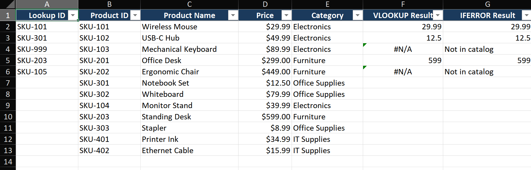
Row 4 now shows "Not in catalog" instead of the ugly #N/A.

Key Techniques and Best Practices

Technique 1 — Use Named Ranges for Self-Documenting Formulas

Formulas with cryptic cell references like $B$2:$E$500 are hard to understand weeks later. Named ranges fix this:

Select range B2:E500. Click in the Name Box (the field to the left of the formula bar that normally shows the cell address).
Type CatalogTable and press Enter. Your range now has a name.
Rewrite the VLOOKUP as: =IFERROR(VLOOKUP(A2, CatalogTable, 3, FALSE), "Not found")
Anyone reading this formula immediately knows CatalogTable is the lookup source — no need to trace cell references.

Technique 2 — Dynamic Column Index with MATCH

Hardcoding 3 as col_index_num breaks when you insert or delete columns. Instead, let MATCH find the right column number automatically:

Assume row 1 (B1:E1) contains headers: "Product ID", "Product Name", "Price", "Category".
Replace the hardcoded 3 with: MATCH("Price", $B$1:$E$1, 0)
Full formula: =IFERROR(VLOOKUP(A2, CatalogTable, MATCH("Price", $B$1:$E$1, 0), FALSE), "Not found")
Now if someone inserts a "Supplier" column between C and D, Price shifts from column 3 to column 4 — but MATCH automatically finds it, so your formula still works.

Technique 3 — The VLOOKUP + COLUMN Trick for Multi-Column Returns

When you need to pull Product Name, Price, AND Category for each lookup ID:

In F2 (Name): =IFERROR(VLOOKUP($A2, CatalogTable, 2, FALSE), "")
In G2 (Price): =IFERROR(VLOOKUP($A2, CatalogTable, 3, FALSE), "")
In H2 (Category): =IFERROR(VLOOKUP($A2, CatalogTable, 4, FALSE), "")
Notice $A2 — the dollar sign locks the column reference to A, but the row (2) adjusts when you copy down. This lets you copy all three formulas across and down in one go.

Common Mistakes (And How to Fix Them Instantly)

Mistake: VLOOKUP returns #N/A even though the data is clearly there.
Fix: Your lookup value and the table's first column have different data types. "00123" (text) ≠ 123 (number). Select the lookup column, go to Data > Text to Columns > Finish to convert text-numbers to real numbers. Or wrap your lookup_value in TEXT(A2, "00000").
Mistake: Formula works for row 2 but breaks when copied to row 3.
Fix: You forgot to lock the table_array with $ signs. Edit F2, select B2:E500 inside the formula, press F4. Should become $B$2:$E$500.
Mistake: VLOOKUP returns the wrong value — it looks almost correct but slightly off.
Fix: You omitted the fourth argument. Without FALSE, VLOOKUP defaults to approximate match. It finds the closest value in a sorted list, which may not be the exact match you want. Always explicitly type FALSE.
Mistake: Inserted a column in the catalog, now all VLOOKUPs are broken.
Fix: Use the MATCH technique from above to make col_index_num dynamic. If you already broke them, use Find & Replace (Ctrl+H) to update the column numbers in bulk.
Mistake: VLOOKUP only returns the first match when there are duplicates.
Fix: VLOOKUP always returns the first match in the lookup column. If you need all matches, switch to INDEX-MATCH with SMALL/IF array formula, or upgrade to XLOOKUP which can return the last match.

Advanced Tips for Power Users

Two-way lookup with VLOOKUP + MATCH: =VLOOKUP(A2, Table, MATCH("Q3", Headers, 0), FALSE) lets you look up both the row (product) and column (quarter). Change "Q3" to "Q4" in one place and get the next quarter's data.
Partial match with wildcards: =VLOOKUP("*"&A1&"*", Table, 2, FALSE) finds rows where the cell contains the text in A1, even if it's buried in a longer string. Useful for searching product descriptions.
Reverse-column lookup with CHOOSE: Need to search a right-side column and return from a left-side column? =VLOOKUP(A2, CHOOSE({1,2}, D2:D100, A2:A100), 2, FALSE) virtually swaps the columns so VLOOKUP sees the search column first.
When to switch to XLOOKUP: If you're on Excel 2021 or Microsoft 365, XLOOKUP eliminates every limitation above — left-to-right, right-to-left, default exact match, built-in error handling. The syntax: =XLOOKUP(A2, SearchColumn, ReturnColumn, "Not found"). Worth learning if your Excel version supports it.

Download Practice Template

Have questions or found an error in this article? Submit Feedback