Power Query Tutorial
What Is Power Query and Why It Changes Everything
Power Query is Excel's built-in ETL (Extract, Transform, Load) engine. In plain English: it's a tool for importing data from almost any source, cleaning and reshaping it automatically, and loading it into your worksheet — with every step recorded and repeatable. If you've ever spent a Friday afternoon manually cleaning a report that arrives in the same messy format every week, Power Query is the solution you've been waiting for.
Unlike macros, Power Query requires no coding. You build transformation steps through a visual interface, and Power Query records them in the M language behind the scenes. When next week's file arrives, one click re-applies all your cleaning steps.
Step-by-Step: Automate a Weekly Sales Report Cleanup
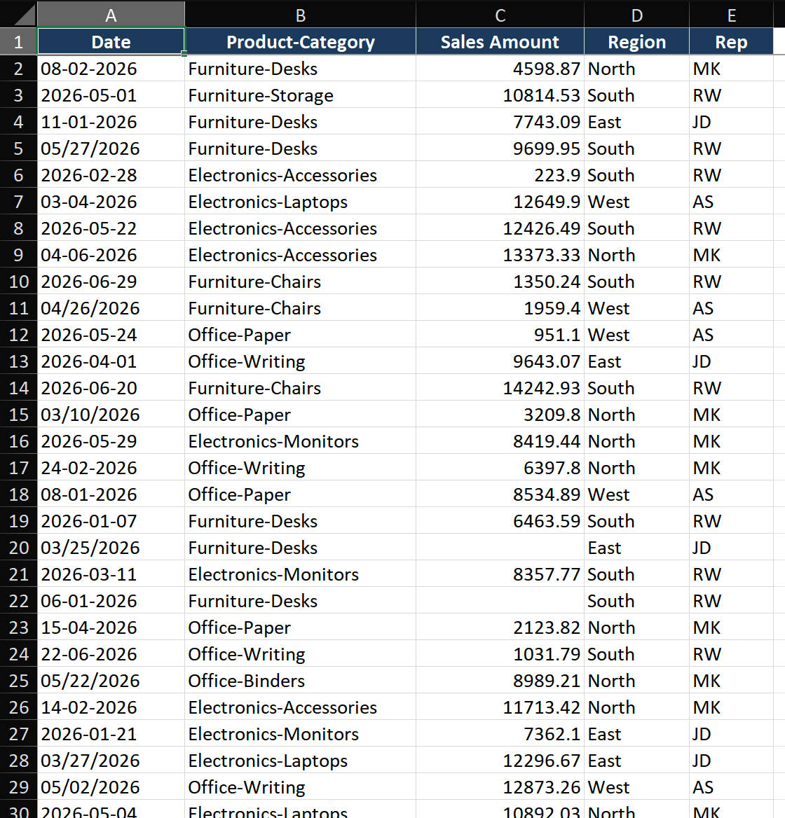
Scenario: Every Monday you receive sales_YYYYMMDD.csv with inconsistent date formats, merged product categories (Category-Subcategory in one column), rows with missing sales amounts, and extra summary rows at the bottom. Build a Power Query that cleans it automatically.
Step 1 — Import the raw data
- Data > Get Data > From File > From Text/CSV.
- Select your sales CSV file. The Navigator previews the data. Note how Power Query already detected delimiters and data types.
- Click Transform Data (not "Load"). This opens the Power Query Editor — all cleaning happens here.
Step 2 — Promote headers and remove garbage rows
- If the first row is headers: Home > Use First Row as Headers. Always do this first — headers enable column-name references in later steps.
- Remove summary rows at the bottom. Filter the date column: click the dropdown, uncheck rows containing text like "Total" or blank values. Or use Home > Remove Rows > Remove Bottom Rows if you know how many extra rows exist.
- Remove completely blank rows: Home > Remove Rows > Remove Blank Rows.
Step 3 — Split the Product Category column
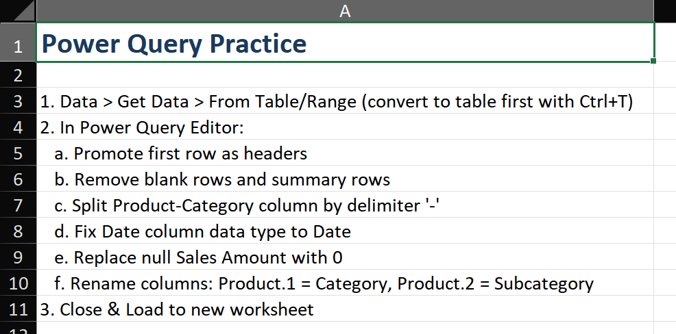
- Your product column contains "Electronics-Accessories" — category hyphen subcategory. You need two columns.
- Select the Product column. Transform > Split Column > By Delimiter.
- Delimiter: Custom, type
-. Split at: Left-most delimiter (important: some subcategories contain hyphens, e.g., "Audio-Visual"). - Click OK. Now you have Product.1 (category) and Product.2 (subcategory). Rename them: right-click headers > Rename.
Step 4 — Fix date format and handle missing values
- Select the Date column. Transform > Data Type > Date. If some dates won't convert (showing Error), click the column dropdown > Replace Errors > enter today's date as fallback, or filter to review those rows.
- For the Sales Amount column: select it, Transform > Replace Values. Value to Find:
null, Replace With:0. This replaces missing sales with zero rather than leaving blanks. - Remove rows where Sales Amount is 0 if they represent meaningless entries (optional): filter Sales Amount > Number Filters > Greater Than > 0.
Step 5 — Load and set up automatic refresh
- Home > Close & Load To. Choose "Table" and "New Worksheet". Click OK.
- Your cleaned data appears in Excel. Now to automate: Data > Queries & Connections (pane on the right).
- Right-click your query > Properties. Check Refresh data when opening the file. Optionally set Refresh every X minutes for live dashboards.
- Next week: save the new CSV with the same name in the same location, open this workbook, and click Data > Refresh All. All cleaning steps replay automatically.
Key Techniques
- Unpivot for analysis-ready data. If your data has months as separate columns (Jan, Feb, Mar), select the descriptive columns and Transform > Unpivot Other Columns. Wide tables become PivotTable-friendly tall tables.
- Merge queries instead of VLOOKUP. Home > Merge Queries joins two tables on matching columns — Power Query's version of VLOOKUP, but handles millions of rows and multiple join types (left, right, full outer, inner, anti).
- Group By for summaries. Transform > Group By to aggregate data (SUM, COUNT, AVERAGE) by category — like a Pivot Table that runs before data hits your worksheet.
- Rename steps for clarity. "Changed Type," "Removed Columns," and "Filtered Rows" become meaningless after 20 steps. Right-click steps > Rename to describe what it does: "Remove blank rows" or "Split full name."
Common Mistakes
- Loading millions of rows unnecessarily. Filter rows before loading. During development, use Home > Keep Rows > Keep Top Rows and remove the filter when ready for full data.
- Not correcting data types explicitly. Power Query guesses types but can be wrong. Select each column and use Home > Data Type to set correctly: Text for IDs, Decimal for currency, Date for dates. Incorrect types are the #1 source of Power Query errors.
- Forgetting Power Query is case-sensitive. Unlike Excel formulas, M language and text filters are case-sensitive. "ABC" doesn't match "abc" in filters or merges unless you apply an uppercase/lowercase transformation first.
- Over-nesting transformations in a single step. Use separate steps for each logical transformation. Independent steps are easier to debug, reorder, and explain to colleagues.
Advanced Tips
- Auto-combine files in a folder. Get Data > From File > From Folder, then click Combine > Combine & Transform. Power Query applies your transformations to every file in the folder. Drop a new file in and refresh — that's weekly report merging automated.
- Parameters for dynamic queries. Home > Manage Parameters lets you create named values (file path, date range, threshold) that users can change without editing the query. Reference parameters in filter steps for self-service reporting.
- Error handling with Try Otherwise. Wrap transformations with
try ... otherwise ...:try Date.FromText([Column]) otherwise null. Prevents one bad cell from failing the entire query.