INDEX-MATCH vs VLOOKUP
The Great Debate: INDEX-MATCH vs. VLOOKUP
VLOOKUP is Excel's most famous lookup function, and INDEX-MATCH is its more powerful, more flexible competitor. This debate has raged in Excel forums for over a decade, and for good reason: choosing the right lookup method directly affects your spreadsheet's reliability, flexibility, and performance.
Spoiler: if you have Excel 2021 or 365, XLOOKUP makes both methods mostly obsolete. But millions of users remain on older versions, and the principles you learn from INDEX-MATCH apply across all Excel functions. Even XLOOKUP users benefit from understanding the underlying mechanism.
Step-by-Step: Convert a VLOOKUP to INDEX-MATCH
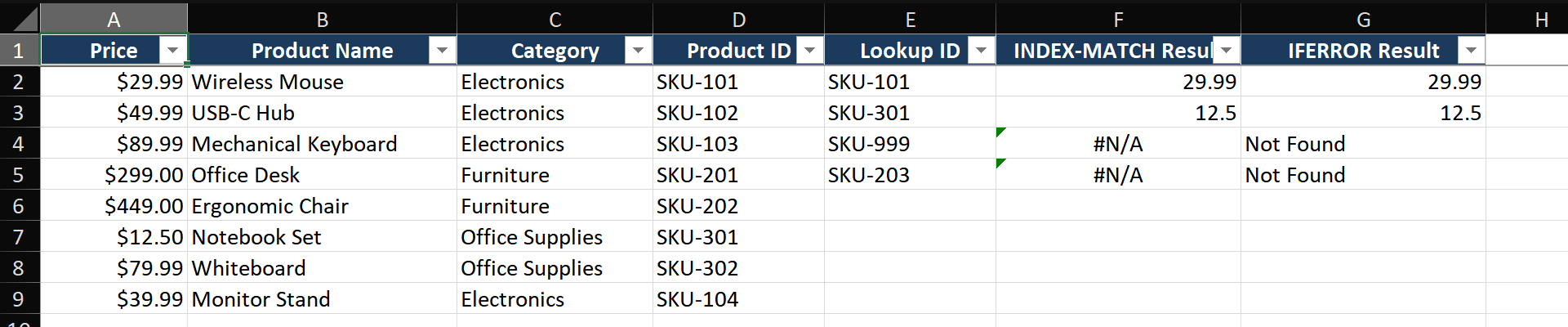
Scenario: You have a product table with Product ID in column D and Price in column A. VLOOKUP fails because the lookup column is to the RIGHT of the return column. You need INDEX-MATCH.
Step 1 — Understand the INDEX-MATCH anatomy
- The formula structure:
=INDEX(return_range, MATCH(lookup_value, lookup_range, 0)) - INDEX(range, row_number) — returns the value from a range at a specific row position.
- MATCH(value, range, 0) — finds the position of a value in a range. The 0 means "exact match."
- Together: MATCH finds the row number, INDEX returns the value at that row in the return column.
Step 2 — Write the formula piece by piece
- In an empty cell, start with MATCH alone to verify it works:
=MATCH(A2, D:D, 0). This should return the row number where the Product ID in A2 is found in column D. - Now wrap it with INDEX to get the price:
=INDEX(A:A, MATCH(A2, D:D, 0)). This returns the price from column A at the row MATCH found. - For production use, lock the ranges:
=INDEX($A$2:$A$1000, MATCH(A2, $D$2:$D$1000, 0)). Never leave whole-column ranges (A:A) unless you enjoy slow calculations.
Step 3 — Handle #N/A errors gracefully
- Wrap the entire formula with IFERROR:
=IFERROR(INDEX($A$2:$A$1000, MATCH(A2, $D$2:$D$1000, 0)), "Not Found"). - Now when a Product ID doesn't exist in the lookup table, you see "Not Found" instead of an ugly error.
- For dashboards, use "" (empty string) instead of "Not Found" for a cleaner look.
When VLOOKUP Wins
- Simplicity and readability. One VLOOKUP formula is easier to read and teach than the INDEX-MATCH combination. For simple lookups where the lookup column is on the left, VLOOKUP is faster to write and easier for colleagues to understand.
- Quick ad-hoc lookups. When you need a one-time lookup and data is already organized with the lookup column first, VLOOKUP is the path of least resistance. Type it and move on.
- Approximate match scenarios. For numeric brackets (tax tiers, commission bands, grading scales), VLOOKUP with TRUE as the fourth argument is straightforward and well-documented.
When INDEX-MATCH Wins
- Lookup column is to the RIGHT of the return column. VLOOKUP only searches left-to-right. INDEX-MATCH doesn't care about column order.
- Inserting or deleting columns. VLOOKUP's col_index_num is hardcoded. Insert a column and all VLOOKUPs referencing columns to the right break. INDEX-MATCH uses actual column references and adjusts correctly.
- Performance on large datasets. INDEX-MATCH can be faster because you can limit the lookup to a single column rather than scanning the entire table array. The difference becomes noticeable above 50,000 rows.
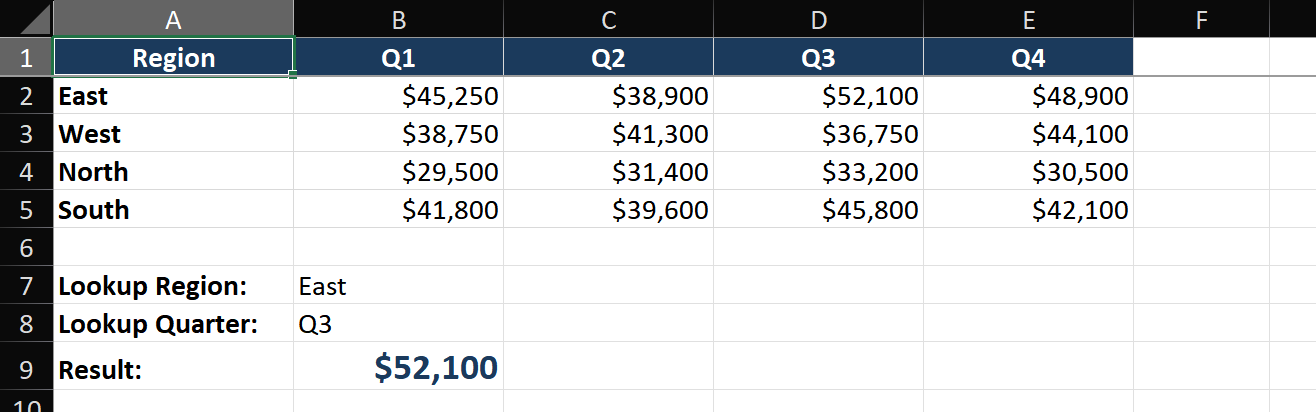
- Two-way (matrix) lookups. INDEX-MATCH-MATCH is a native capability:
=INDEX(data_range, MATCH(row_value, row_headers, 0), MATCH(col_value, col_headers, 0)).
Common Mistakes
- Forgetting VLOOKUP can't look left. This is the #1 frustration. If you find yourself rearranging columns just to make VLOOKUP work, you're fighting the wrong battle — switch to INDEX-MATCH.
- VLOOKUP accidentally using approximate match. The fourth argument defaults to TRUE if omitted. Forgetting to add FALSE produces "close enough" results that look correct but are subtly wrong. Always write FALSE explicitly.
- Not locking MATCH ranges in INDEX-MATCH.
=INDEX(D:D, MATCH(A2, B:B, 0))is fragile. Lock the ranges:=INDEX($D$2:$D$100, MATCH(A2, $B$2:$B$100, 0)). - Assuming INDEX-MATCH is always faster. On small datasets (under 1,000 rows), the performance difference is negligible. Simplicity often beats a marginal speed gain.
Advanced Tips
- INDEX-MATCH-MATCH for dynamic column selection: Create a dropdown for column name, then
=INDEX(data, MATCH(row_val, row_col, 0), MATCH(dropdown, headers, 0)). One formula becomes a self-service lookup tool. - INDEX-MATCH for last occurrence:
=INDEX(return_range, MATCH(2, 1/(lookup_range=value), 1))returns the last match, not the first. Useful for finding a customer's most recent transaction. - Array INDEX-MATCH for multiple criteria:
=INDEX(return_range, MATCH(1, (range1=A2)*(range2=B2), 0))entered with Ctrl+Shift+Enter. Returns the first row matching multiple conditions without helper columns.