Data Cleaning in Excel
Why Clean Data Is Non-Negotiable
Dirty data is Excel productivity's silent killer. Extra spaces, inconsistent formats, duplicate records, and missing values break your formulas, confuse your Pivot Tables, and lead to decisions based on wrong numbers. Research consistently shows data professionals spend 60-80% of their time cleaning data — not analyzing it.
The good news: Excel has powerful built-in tools designed specifically for data cleaning. You don't need to manually scan thousands of rows. This guide covers the core techniques that will cut your data prep time in half.
Step-by-Step: Clean a Real Dataset
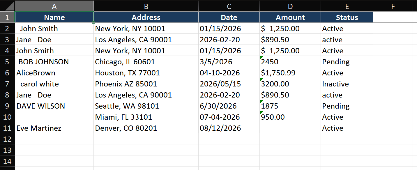
Scenario: You received a CSV export from a legacy system. Column A has names with extra spaces, column B has "City, State ZIP" combined in one cell, column C has dates in mixed formats, and there are duplicate rows scattered throughout.
Step 1 — Always work on a copy first
- Right-click the sheet tab > Move or Copy > Create a copy. Name the copy "Cleaned".
- Never clean the only version of your data. If a cleaning step goes wrong, you can always return to the original.
Step 2 — Remove duplicate rows
- Click any cell inside the data, press Ctrl+A to select all.
- Go to Data > Remove Duplicates.
- Uncheck columns that shouldn't define uniqueness (like timestamps that differ even for the same record). Check only the key columns: Name and Date, for example.
- Click OK. Excel reports how many duplicates were removed and how many unique rows remain.
Step 3 — Clean text with TRIM and CLEAN
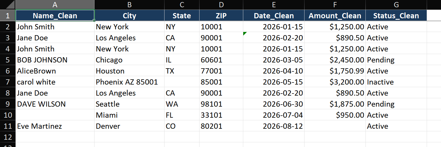
- Insert a new column next to the Name column (right-click column B > Insert). Label it "Name_Clean".
- In the first data row, enter:
=TRIM(CLEAN(A2)) - Double-click the fill handle to copy down. TRIM removes leading, trailing, and excess spaces. CLEAN removes non-printable characters (common in system exports).
- Copy the cleaned column, right-click the original > Paste Special > Values to replace the formulas with clean text. Delete the helper column.
Step 4 — Split "City, State ZIP" using Text to Columns
- Select the combined address column. Data > Text to Columns.
- Choose Delimited, click Next. Check Comma as the delimiter.
- Preview shows the split. Click Next.
- For each destination column, set the data format: "City" as Text, "State ZIP" as Text. Click Finish.
- Now split "State ZIP" again: select it, Text to Columns > Delimited > Space. You now have three clean columns: City, State, ZIP.
Step 5 — Standardize dates
- Select the dates column. Data > Text to Columns > Delimited > uncheck all delimiters > Next.
- Under "Column data format," select Date and choose the format that matches your data (MDY, DMY, etc.).
- Click Finish. Excel converts all dates to a consistent, sortable format.
- For dates that still look wrong, apply a uniform format: Ctrl+1 > Number > Date > pick your desired display format.
Key Techniques
Technique 1 — Flash Fill for pattern recognition
Flash Fill (Ctrl+E) watches your manual edits and auto-completes the rest based on detected patterns.
- Next to a column of full names, type the first name from the first cell. Press Enter.
- Start typing the second name. Excel shows a gray preview of suggested completions.
- Press Ctrl+E to accept. Flash Fill extracts first names from all rows instantly. Works for splitting, combining, formatting, and extracting parts of text.
Technique 2 — Find & Replace with wildcards
- Press Ctrl+H to open Find and Replace.
- To remove everything after a hyphen in product codes: Find
-*, Replace with nothing. *matches any number of characters.?matches exactly one character.- Always click Find All first to preview matches before committing the replace.
Common Mistakes
- Cleaning the original file. Always work on a copy. Cleaning is often irreversible — TRIM and Text to Columns destroy the original data format.
- Deleting rows with missing data without analysis. Blank cells may indicate a data collection issue, not useless records. Check if missing data is random or systematic before deleting.
- TRIM doesn't remove non-breaking spaces (char 160). Web data often contains these. Use
=SUBSTITUTE(A2, CHAR(160), " ")before TRIM to completely clean whitespace. - Excel strips leading zeros from numbers. For ZIP codes, product IDs, or employee numbers, format the column as Text before importing, or use
=TEXT(A2, "00000")to restore leading zeros.
Advanced Tips
- Build a data quality dashboard: Use COUNTA, COUNTBLANK, and conditional formatting to create a summary showing completeness (%) for each column. Add data validation rules with COUNTIF to flag invalid entries automatically.
- Power Query for repeatable cleaning: Data > Get Data > From Table/Range opens Power Query. Build cleaning steps once (trim, split, filter, replace), then each week just drop in the new file and Refresh — all steps auto-replay.
- Fuzzy matching in Power Query: The Fuzzy Merge option matches similar-but-not-identical text — perfect for reconciling "IBM Corp." with "International Business Machines" when merging tables from different systems.
- UNIQUE and SORT for quick dedup reference: In Excel 365,
=SORT(UNIQUE(A2:A1000))returns an alphabetically sorted list of all distinct values — instant reference for what's actually in each column.