Conditional Formatting Tricks

Make Your Data Speak Visually

Conditional Formatting transforms raw numbers into visual stories. Instead of scanning thousands of cells for outliers, trends, or patterns, Excel automatically highlights them — red for negative numbers, green for targets met, color gradients for performance ranges. It's Excel's most underutilized feature for making reports instantly readable.

The concept: you define a rule, and Excel applies formatting only when that rule is true. But the depth you can achieve — from simple highlight rules to formula-driven dynamic formatting — is what separates basic spreadsheets from professional dashboards.

Excel spreadsheet with three Conditional Formatting examples side by side: (1) Data bars in a Sales column showing relative bar lengths, (2) Color scale heatmap across a matrix of monthly sales figures from green (high) to red (low), (3) Icon sets with green-yellow-red traffic lights next to KPI numbers. — Fig 1. — Three common Conditional Formatting patterns in action: data bars (cell-level bar charts), color scales (heatmaps), and icon sets (KPI indicators).

Step-by-Step: Apply Your First Conditional Formatting Rule

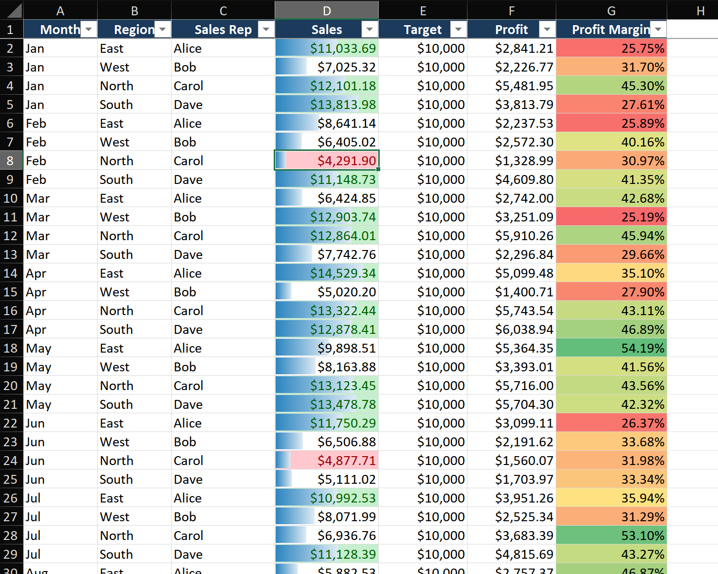
Scenario: You have a sales performance table. Column D shows monthly sales. You want cells over $10,000 highlighted green, and cells below $5,000 highlighted red.

Step 1 — Select the data range

Click cell D2, then press Ctrl+Shift+Down Arrow to select the entire Sales column (D2:D200).
Do NOT select the header cell D1 — Conditional Formatting rules should apply to data cells only.
Confirm your selection in the Name Box shows something like D2:D200.

Step 2 — Apply the first rule (high values → green)

Go to Home > Conditional Formatting > Highlight Cells Rules > Greater Than.
In the dialog, type 10000 in the left box.
From the right dropdown, choose Green Fill with Dark Green Text (or pick Custom Format to choose your own).
Click OK. All cells above $10,000 are now green.

Step 3 — Add a second rule (low values → red)

With D2:D200 still selected, go to Conditional Formatting > Highlight Cells Rules > Less Than.
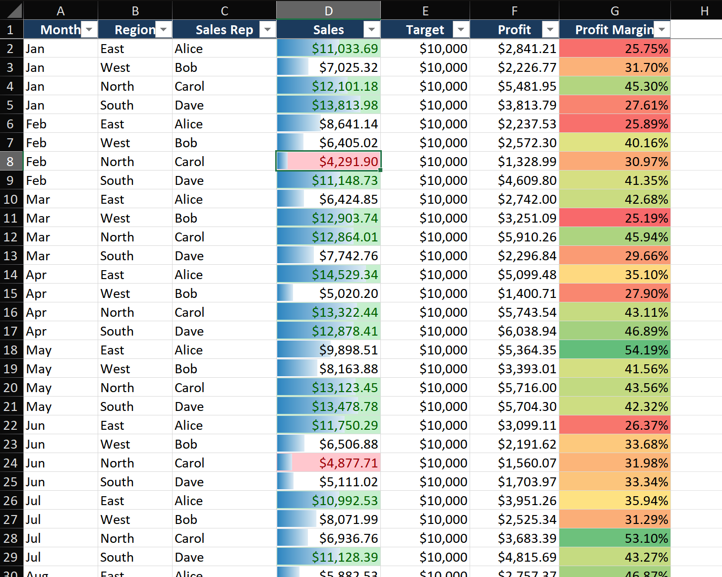
Type 5000, choose Light Red Fill with Dark Red Text. Click OK.
Now you have a two-color system: green for high performers, red for low performers, and white for everything in between.

Sales column with Conditional Formatting applied: cells above $10,000 show green fill, cells below $5,000 show red fill, middle-range values remain white. The Conditional Formatting Rules Manager dialog is open showing both rules in order. — Fig 2. — Result after applying both rules. Green = above target, Red = below threshold, White = middle range.

Step 4 — Manage and reorder rules

Go to Conditional Formatting > Manage Rules.
Set "Show formatting rules for" to "This Worksheet" to see all rules.
Rules are evaluated top-to-bottom. The first rule that matches wins. Use the up/down arrows to reorder if needed.
Check "Stop If True" to prevent lower rules from overriding a matched rule.

Key Techniques

Technique 1 — Data Bars for in-cell visual comparisons

Select your numeric column. Conditional Formatting > Data Bars > pick a solid fill color.
Each cell now contains a horizontal bar proportional to its value — the largest value fills the cell, others scale accordingly.
Pro tip: Manage Rules > Edit Rule > check "Show Bar Only" to hide the numbers and show only the bars.

Technique 2 — Formula rules for whole-row highlighting

Want to highlight entire rows based on a single cell's value?

Select your entire table (A2:F200).
Conditional Formatting > New Rule > Use a formula.
Enter: =$D2>10000 — the $ locks column D, but row 2 adjusts for each row.
Click Format, choose a Fill color. Now any row where column D exceeds $10,000 turns that color entirely.

New Formatting Rule dialog showing 'Use a formula to determine which cells to format' selected. Formula box contains =$D2>10000. Below, a preview shows the green fill that will be applied. The background spreadsheet shows entire rows highlighted green where column D exceeds $10,000. — Fig 3. — The formula rule dialog. The $ before D locks the column reference so the rule checks only column D for each row.

Technique 3 — Color Scales for heatmaps

Select a range of numbers. Conditional Formatting > Color Scales > Green-White-Red.
High values turn green, low values turn red, middle values are white with smooth gradients in between.
For a two-color scale showing deviation from a midpoint (like 0), use More Rules > set Midpoint to 0.

Common Mistakes

Applying rules to entire columns (D:D). This evaluates millions of empty cells, slowing your workbook to a crawl. Limit rules to your actual data range or use Excel Tables (rules auto-expand with Tables).
Too many overlapping rules. When multiple rules apply, the first TRUE match wins. Five overlapping rules create confusing behavior. Keep rule sets minimal.
Forgetting $ signs in formula rules. =D2>10000 looks correct, but when applied to range A2:F200, Excel shifts the column reference. Use =$D2>10000 to always check column D.
Copying cells duplicates rules. Paste operations can multiply Conditional Formatting rules. Check Manage Rules periodically and delete duplicate or fragmented rules.

Advanced Tips

Gantt chart with Conditional Formatting: Set up a timeline grid with dates as column headers and tasks as rows. Apply formula rule: =AND(G$1>=$C2, G$1<=$D2) where row 1 is dates, C is start, D is end. Instantly visualizes project timelines.
Dynamic search highlighting: Create a search cell (E1). Apply formula to data range: =ISNUMBER(SEARCH($E$1, A2)). Typing in E1 instantly highlights all matching cells — live search without VBA.
Duplicate and unique value detection: Use =COUNTIF($A$2:$A$1000, A2)>1 to highlight duplicates. Use =COUNTIF($A$2:$A$1000, A2)=1 for unique values only.
Weekend and holiday coloring: =WEEKDAY($A2, 2)>5 highlights weekends. Combine with a named range "Holidays" and =COUNTIF(Holidays, $A2)>0 for professional calendar formatting.

Download Practice Template

Have questions or found an error in this article? Submit Feedback